Parsing a Hand-drawn Hash Game

In this tutorial I will show you how to parse a hand-drawn hash game with Computer Vision techniques to determine who’s the winner (if any). See the example below:

For this tutorial we are going to use OpenCV 3.2.

Basically, in order to perform what we intend, we need first to detect where are the ‘x’ and the ‘o’, and later check if they are aligned in such way that indicates a win (aligned on horizontal, vertical or diagonal).

Check the image below:

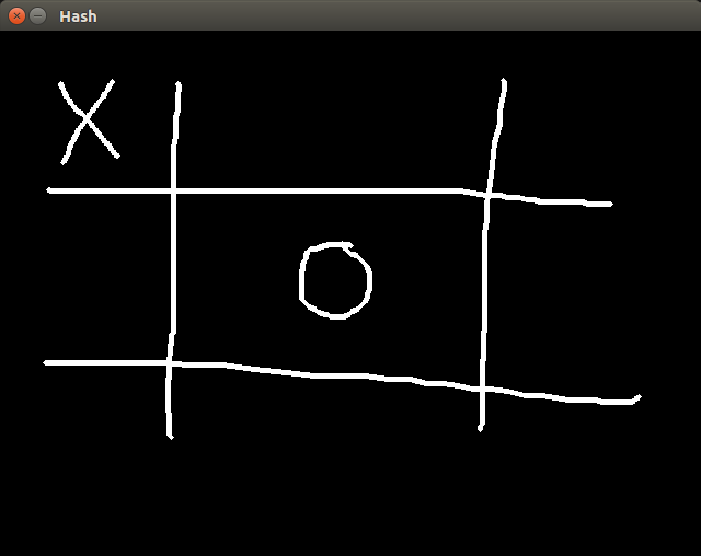
This is the kind of image we want to deal with. In order to detect each element of that image, we need to segment them. We can do that easily with the OpenCV connectedComponents function. What it does is very simple: For each white pixel of a binary image it associates a label indicating to which group (or connected component) the pixel belongs to. A connected component is a set of white pixels where each pixel is a neighbor of some other white pixel within the same component.

For the image above, it would output three connected components: the hash, the ‘x’ symbol and the ‘o’ symbol. Once we have all them three apart, the detection process becomes much easier.

hash.cpp

#include <vector>
#include <opencv2/core/core.hpp>
#include <opencv2/highgui/highgui.hpp>
#include <opencv2/imgproc/imgproc.hpp>

cv::Mat gImg;

std::vector<std::pair<cv::Mat, cv::Rect> > getConnectedComponents()
{
  cv::Mat labels(gImg.rows, gImg.cols, CV_32S);
  cv::connectedComponents(gImg, labels);
  int *label = (int*)labels.data;
  
  std::map<int, std::vector<cv::Point2i> > components;
  for (int y = 0; y < labels.rows; y++)
  {
      for (int x = 0; x < labels.cols; x++)
      {
          if (*label > 0) // not background
          {
              components[*label].push_back(cv::Point2i(x, y));
          }
          ++label;
      }
  }
  
  std::vector<std::pair<cv::Mat, cv::Rect> > connectedComponents;
  std::vector<cv::Mat> imgs;
  std::vector<cv::Rect> rects;
  for (auto it = components.begin(); it != components.end(); ++it)
  {
      cv::Rect boundingRect;
      cv::Mat img = getComponentImg(it->second, boundingRect);
      connectedComponents.push_back(std::make_pair(img, boundingRect));
  }
  return connectedComponents;
}

int main()
{
  gImg = cv::imread("hash1.png", 0);
}

Ok! In order to call the connectedComponents function, we need to pass a image of same dimension of the input image. It will store the label associated to each pixel. Then it iterates over each pixel of the label image and saves the position in a map that associates a label to a vector of positions. After that, we want to get bounding rect and a image containing only the pixels of a determined component. For that I’m calling the getComponentImg function. Let’s see how it’s implemented:

hash.cpp

cv::Mat getComponentImg(const std::vector<cv::Point2i> &pixels, cv::Rect &boundingRect)
{
  int minX = INT_MAX, maxX = INT_MIN, minY = INT_MAX, maxY = INT_MIN;
  for (size_t i = 0; i < pixels.size(); i++)
  {
      cv::Point2i pixel = pixels[i];
      if (pixel.x < minX) minX = pixel.x;
      if (pixel.x > maxX) maxX = pixel.x;
      if (pixel.y < minY) minY = pixel.y;
      if (pixel.y > maxY) maxY = pixel.y;
  }
  boundingRect = cv::Rect(minX, minY, maxX - minX + 20, maxY - minY + 20);
  cv::Mat img = cv::Mat::zeros(boundingRect.height, boundingRect.width, CV_8U);
  for (size_t i = 0; i < pixels.size(); i++)
  {
      cv::Point2i pixel = pixels[i] - boundingRect.tl() + cv::Point2i(10, 10);
      img.at<uchar>(pixel.y, pixel.x) = static_cast<uchar>(255);
  }
  return img;
}

Very straight-forward, since we already have a list containing all the positions of the elements within the connected component. All we need to that is get the min and dimensions of those pixels, then calculate a bounding rect, creating a image of the dimension of the bounding rect, iterate over each position and set it in the image we just created.

Ok!!! Now we have each element separated, as we can see below:

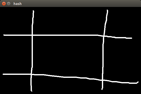
How can we accomplish the detection now? Well, there are many many ways. I’m going to diver the machine learning path. We will train a neural network with many examples of ‘x’ and ‘o’, in such way that the next time the user draw any of them, the classifier will know which of them the user drew. Once we know that, we just need to check the alignment and ta-dah! Very simple.

Obviously, we can’t train with the raw images (because their dimension vary. we could draw at a time a big ‘x’ and then a small ‘x’. we could resize, we then we were performing distortions). We need a feature descriptor. In this example, I’m going to user a Histogram of oriented gradients, because it makes the most sense, since the ‘x’ symbol have a very different gradient than a ‘o’.

Ok, ok, calm down!!! What is a gradient you are talking about, exactly?

In Calculus, gradient is the rate of change of a function at a given point. Just see image below:

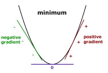
This represent the gradient of the f(x) = x² function. Obviously, since we are squaring ‘x’, higher values of ‘x’ outputs much higher values of f(x) than lower values of ‘x’. Thus, the gradient on the left side is negative (since it is the direction which f(x) changes most) and has a increasing values as ‘x’ increase. The same can be said about the right side, but with oposite direction.

But what does it have to do with images? Can we calculate gradients of images? Of course yes!!! Images are nothing else than 2D discrete functions.

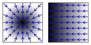
Since we can’t know exactly the f(x) for a image, we need to calculate an approximation for the gradient, calculating the difference between two neighbors pixels for each dimension. In fact, this is exactly what the Sobel filter does.

In possession of both gradients on ‘x’ and ‘y’ direction, we can calculate the angle to which the gradient is pointing to by taking the inverse tangent of x and y. For the ‘x’ symbol, the gradient will point alongside the edges (thus only two directions) while for the ‘o’ symbol, the gradient will tangent each pixel, and since it’s a ellipse, we are going to have gradients pointing to many directions. That way we can distinguish a symbol from another.

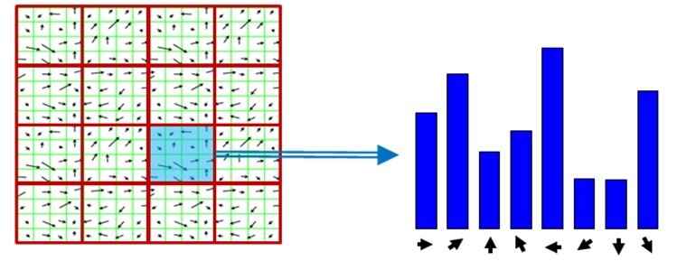
Enough talking!! Let’s see the code:

hash.cpp

std::vector<float> getHistogramOfOrientations(cv::Mat &component)
{
  std::vector<float> histogramOfOrientations(HISTOGRAM_SIZE, 0.0f);
  cv::Mat gradX, gradY;
  cv::Sobel(component, gradX, CV_32F, 1, 0, 3, 1, 0, cv::BORDER_DEFAULT);
  cv::Sobel(component, gradY, CV_32F, 0, 1, 3, 1, 0, cv::BORDER_DEFAULT);
  float *gradXPtr = (float*)gradX.data;
  float *gradYPtr = (float*)gradY.data;
  float sum = 0;
  for (int i = 0, end = gradX.rows * gradX.cols; i < end; i++)
  {
      float x = *gradXPtr;
      float y = *gradYPtr;
      float orientation = (std::atan2(y, x) + M_PI) * 180 / M_PI;
      float norm = std::sqrt(std::pow(x, 2) + std::pow(y, 2));
      histogramOfOrientations[(int)(orientation / (360.0f / HISTOGRAM_SIZE)) % HISTOGRAM_SIZE] += norm;
      sum += norm;
      ++gradXPtr;
      ++gradYPtr;
  }
  for (int i = 0; i < HISTOGRAM_SIZE; i++)
  {
      histogramOfOrientations[i] /= sum;
  }
  return histogramOfOrientations;    
}

Set a variable named HISTOGRAM_SIZE to determine the number of bins of the histogram (lower values are better, due to the curse of dimensionality thing).

Training the classifier is pretty straight-forward also, once we have the histograms of each sample:

hash.cpp

void learnClassifier()
{
  cv::Mat trainSamples(3 * NUM_DRAWINGS, HISTOGRAM_SIZE, CV_32F);
  cv::Mat trainResponses = cv::Mat::zeros(3 * NUM_DRAWINGS, 3, CV_32F);
  for (int classId = 0; classId < 3; classId++)
  {
      for (int sampleId = 0; sampleId < NUM_DRAWINGS; sampleId++)
      {
          for (int featureId = 0; featureId < HISTOGRAM_SIZE; featureId++)
          {
              trainSamples.at<float>(classId * NUM_DRAWINGS + sampleId, featureId) = gFeatures[classId][sampleId][featureId];
          }
          trainResponses.at<float>(classId * NUM_DRAWINGS + sampleId, classId) = 1.0f;
      }
  }
  gNeuralNetwork = cv::ml::ANN_MLP::create();
  std::vector<int> layerSizes = { HISTOGRAM_SIZE, HISTOGRAM_SIZE * 4, 3 };
  gNeuralNetwork->setLayerSizes(layerSizes);
  gNeuralNetwork->setActivationFunction(cv::ml::ANN_MLP::SIGMOID_SYM);
  gNeuralNetwork->train(trainSamples, cv::ml::ROW_SAMPLE, trainResponses);
  gNeuralNetwork->save("mlp.yaml");
}

NUM_DRAWINGS is the number of samples for each class. The samples are stored in a 3D array named gFeatures. Pay special attention to the layerSizes variables. It’s the variable which determines the number of neurons for each layer. It has a profound impact in the performance of a neural network.

Finally, we just need to get the label associated to each component, group them and check their alignment.

hash.cpp

bool checkWinner(const std::vector<cv::Rect> &cells)
{
  if (cells.size() == 3)
  {
      std::vector<cv::Rect> horizontalLine = { cells[0] };
      std::vector<cv::Rect> verticalLine = { cells[0] };
      std::vector<cv::Rect> diagonal = { cells[0] };
      int x1s = cells[0].x;
      int x1e = cells[0].x + cells[0].width;
      int y1s = cells[0].y;
      int y1e = cells[0].y + cells[0].height;
      for (size_t i = 1; i < cells.size(); i++)
      {
          int x2s = cells[i].x;
          int x2e = cells[i].x + cells[i].width;
          int y2s = cells[i].y;
          int y2e = cells[i].y + cells[i].height;
          if (x2s >= x1s && x2s <= x1e || x1s >= x2s && x1s <= x2e)
          {
              verticalLine.push_back(cells[i]);
          }
          else if (y2s >= y1s && y2s <= y1e || y1s >= y2s && y1s <= y2e)
          {
              horizontalLine.push_back(cells[i]);
          }
          else if (y2s > diagonal[i].y && x2s > diagonal[i].x
              && y2e > diagonal[i].y + diagonal[i].height && x2e > diagonal[i].x + diagonal[i].width)
          {
              diagonal.push_back(cells[i]);
          }
          if (horizontalLine.size() == 3)
          {
              drawHorizontalLine(horizontalLine);
              return true;
          }
          if (verticalLine.size() == 3)
          {
              drawVerticalLine(verticalLine);
              return true;
          }
          if (diagonal.size() == 3)
          {
              drawDiagonalLine(diagonal);
              return true;
          }
      }
  }
  return false;
}

In the final code I included many more details, such as asking the user to draw some examples of ‘x’ and ‘o’ so the neural network have samples to train on. See it below:

FINAL CODE

hash.cpp

#include <iostream>
#include <map>
#include <fstream>
#include <opencv2/core/core.hpp>
#include <opencv2/highgui/highgui.hpp>
#include <opencv2/imgproc/imgproc.hpp>
#include <opencv2/ml/ml.hpp>

#define STATE_DRAW_X 0
#define STATE_DRAW_O 1
#define STATE_PLAY 2
#define NUM_DRAWINGS 5
#define HISTOGRAM_SIZE 8

bool gMouseDown = false;
cv::Mat gImg;
cv::Point2i gMousePosition;
std::map<char, std::vector<std::vector<float> > > gFeatures;
int gCurrentState = STATE_DRAW_X;
cv::Ptr<cv::ml::ANN_MLP> gNeuralNetwork;

std::vector<float> getHistogramOfOrientations(cv::Mat &component)
{
  std::vector<float> histogramOfOrientations(HISTOGRAM_SIZE, 0.0f);
  cv::Mat gradX, gradY;
  cv::Sobel(component, gradX, CV_32F, 1, 0, 3, 1, 0, cv::BORDER_DEFAULT);
  cv::Sobel(component, gradY, CV_32F, 0, 1, 3, 1, 0, cv::BORDER_DEFAULT);
  float *gradXPtr = (float*)gradX.data;
  float *gradYPtr = (float*)gradY.data;
  float sum = 0;
  for (int i = 0, end = gradX.rows * gradX.cols; i < end; i++)
  {
      float x = *gradXPtr;
      float y = *gradYPtr;
      float orientation = (std::atan2(y, x) + M_PI) * 180 / M_PI;
      float norm = std::sqrt(std::pow(x, 2) + std::pow(y, 2));
      histogramOfOrientations[(int)(orientation / (360.0f / HISTOGRAM_SIZE)) % HISTOGRAM_SIZE] += norm;
      sum += norm;
      ++gradXPtr;
      ++gradYPtr;
  }
  for (int i = 0; i < HISTOGRAM_SIZE; i++)
  {
      histogramOfOrientations[i] /= sum;
  }
  return histogramOfOrientations;    
}

cv::Mat getComponentImg(const std::vector<cv::Point2i> &pixels, cv::Rect &boundingRect)
{
  int minX = INT_MAX, maxX = INT_MIN, minY = INT_MAX, maxY = INT_MIN;
  for (size_t i = 0; i < pixels.size(); i++)
  {
      cv::Point2i pixel = pixels[i];
      if (pixel.x < minX) minX = pixel.x;
      if (pixel.x > maxX) maxX = pixel.x;
      if (pixel.y < minY) minY = pixel.y;
      if (pixel.y > maxY) maxY = pixel.y;
  }
  boundingRect = cv::Rect(minX, minY, maxX - minX + 20, maxY - minY + 20);
  cv::Mat img = cv::Mat::zeros(boundingRect.height, boundingRect.width, CV_8U);
  for (size_t i = 0; i < pixels.size(); i++)
  {
      cv::Point2i pixel = pixels[i] - boundingRect.tl() + cv::Point2i(10, 10);
      img.at<uchar>(pixel.y, pixel.x) = static_cast<uchar>(255);
  }
  return img;
}

std::vector<std::pair<cv::Mat, cv::Rect> > getConnectedComponents()
{
  cv::Mat labels(gImg.rows, gImg.cols, CV_32S);
  cv::connectedComponents(gImg, labels);
  int *label = (int*)labels.data;
  
  std::map<int, std::vector<cv::Point2i> > components;
  for (int y = 0; y < labels.rows; y++)
  {
      for (int x = 0; x < labels.cols; x++)
      {
          if (*label > 0) // not background
          {
              components[*label].push_back(cv::Point2i(x, y));
          }
          ++label;
      }
  }
  
  std::vector<std::pair<cv::Mat, cv::Rect> > connectedComponents;
  std::vector<cv::Mat> imgs;
  std::vector<cv::Rect> rects;
  for (auto it = components.begin(); it != components.end(); ++it)
  {
      cv::Rect boundingRect;
      cv::Mat img = getComponentImg(it->second, boundingRect);
      connectedComponents.push_back(std::make_pair(img, boundingRect));
  }
  return connectedComponents;
}

int getComponentLabel(cv::Mat &component)
{
  std::vector<float> histogram = getHistogramOfOrientations(component);
  cv::Mat sample(1, HISTOGRAM_SIZE, CV_32F, histogram.data());
  cv::Mat predictions;
  gNeuralNetwork->predict(sample, predictions);
  int label = 0;
  for (int i = 1; i < 2; i++)
  {
      if (predictions.at<float>(i) > predictions.at<float>(label))
      {
          label = i;
      }
  }
  return label;
}

void learnClassifier()
{
  cv::Mat trainSamples(2 * NUM_DRAWINGS, HISTOGRAM_SIZE, CV_32F);
  cv::Mat trainResponses = cv::Mat::zeros(2 * NUM_DRAWINGS, 2, CV_32F);
  for (int classId = 0; classId < 2; classId++)
  {
      for (int sampleId = 0; sampleId < NUM_DRAWINGS; sampleId++)
      {
          for (int featureId = 0; featureId < HISTOGRAM_SIZE; featureId++)
          {
              trainSamples.at<float>(classId * NUM_DRAWINGS + sampleId, featureId) = gFeatures[classId][sampleId][featureId];
          }
          trainResponses.at<float>(classId * NUM_DRAWINGS + sampleId, classId) = 1.0f;
      }
  }
  gNeuralNetwork = cv::ml::ANN_MLP::create();
  std::vector<int> layerSizes = { HISTOGRAM_SIZE, HISTOGRAM_SIZE * 2, 2 };
  gNeuralNetwork->setLayerSizes(layerSizes);
  gNeuralNetwork->setActivationFunction(cv::ml::ANN_MLP::SIGMOID_SYM);
  gNeuralNetwork->train(trainSamples, cv::ml::ROW_SAMPLE, trainResponses);
  gNeuralNetwork->save("mlp.yaml");
}

void drawHorizontalLine(const std::vector<cv::Rect> &cells)
{
  int minX = 0, maxX = 0;
  for (size_t i = 1; i < cells.size(); i++)
  {
      if (cells[i].x < cells[minX].x) minX = i;
      if (cells[i].x > cells[maxX].x) maxX = i;
  }
  cv::Point2i p1(cells[minX].x, cells[minX].y + cells[minX].height / 2);
  cv::Point2i p2(cells[maxX].x + cells[maxX].width, cells[maxX].y + cells[maxX].height / 2);
  cv::Mat img(gImg.rows, gImg.cols, CV_8UC3);
  cv::line(gImg, p1, p2, cv::Scalar(255, 0, 0), 3);
}

void drawVerticalLine(const std::vector<cv::Rect> &cells)
{
  int minY = 0, maxY = 0;
  for (size_t i = 1; i < cells.size(); i++)
  {
      if (cells[i].y < cells[minY].y) minY = i;
      if (cells[i].y > cells[maxY].y) maxY = i;
  }
  cv::Point2i p1(cells[minY].x + cells[minY].width / 2, cells[minY].y);
  cv::Point2i p2(cells[maxY].x + cells[maxY].width / 2, cells[maxY].y + cells[maxY].height);
  cv::line(gImg, p1, p2, cv::Scalar(255, 0, 0), 3);
}

void drawDiagonalLine(const std::vector<cv::Rect> &cells)
{
  int minY = 0, maxY = 0;
  for (size_t i = 1; i < cells.size(); i++)
  {
      if (cells[i].y < cells[minY].y) minY = i;
      if (cells[i].y > cells[maxY].y) maxY = i;
  }
  cv::Point2i p1(cells[minY].x, cells[minY].y);
  cv::Point2i p2(cells[maxY].x + cells[maxY].width, cells[maxY].y + cells[maxY].height);
  cv::line(gImg, p1, p2, cv::Scalar(255, 0, 0), 3);
}

bool checkWinner(const std::vector<cv::Rect> &cells)
{
  if (cells.size() == 3)
  {
      std::vector<cv::Rect> horizontalLine = { cells[0] };
      std::vector<cv::Rect> verticalLine = { cells[0] };
      std::vector<cv::Rect> diagonal = { cells[0] };
      int x1s = cells[0].x;
      int x1e = cells[0].x + cells[0].width;
      int y1s = cells[0].y;
      int y1e = cells[0].y + cells[0].height;
      for (size_t i = 1; i < cells.size(); i++)
      {
          int x2s = cells[i].x;
          int x2e = cells[i].x + cells[i].width;
          int y2s = cells[i].y;
          int y2e = cells[i].y + cells[i].height;
          if (x2s >= x1s && x2s <= x1e || x1s >= x2s && x1s <= x2e)
          {
              verticalLine.push_back(cells[i]);
          }
          else if (y2s >= y1s && y2s <= y1e || y1s >= y2s && y1s <= y2e)
          {
              horizontalLine.push_back(cells[i]);
          }
          else if (y2s > diagonal[i].y && x2s > diagonal[i].x
              && y2e > diagonal[i].y + diagonal[i].height && x2e > diagonal[i].x + diagonal[i].width)
          {
              diagonal.push_back(cells[i]);
          }
          if (horizontalLine.size() == 3)
          {
              drawHorizontalLine(horizontalLine);
              return true;
          }
          if (verticalLine.size() == 3)
          {
              drawVerticalLine(verticalLine);
              return true;
          }
          if (diagonal.size() == 3)
          {
              drawDiagonalLine(diagonal);
              return true;
          }
      }
  }
  return false;
}

void processHash()
{
  std::vector<std::pair<cv::Mat, cv::Rect> >  components = getConnectedComponents();
  std::vector<cv::Rect> xs;
  std::vector<cv::Rect> os;
  size_t biggestComponent = 0;
  for (size_t i = 1; i < components.size(); i++)
  {
      if (components[i].first.rows * components[i].first.cols >
          components[biggestComponent].first.rows * components[biggestComponent].first.cols)
      {
          biggestComponent = i;
      }
  }
  for (size_t i = 0; i < components.size(); i++)
  {
      if (i == biggestComponent) continue; // the biggest component is obviously the hash
      int label = getComponentLabel(components[i].first);
      if (label == 0) xs.push_back(components[i].second);
      else if (label == 1) os.push_back(components[i].second);
      std::cout << label << std::endl;
  }
  if (!checkWinner(xs))
  {
      checkWinner(os);
  }
  std::cout << std::endl;
}

void addDrawingFeature()
{
  std::vector<std::pair<cv::Mat, cv::Rect> > components = getConnectedComponents();
  if (components.empty()) // user didn't draw anything
  {
      return;
  }
  else if (components.size() > 1) // user drew more than one thing, then select the biggest thing
  {
      int biggestComponent = 0;
      for (size_t i = 1; i < components.size(); i++)
      {
          if (components[i].first.rows * components[i].first.cols >
              components[biggestComponent].first.rows * components[biggestComponent].first.cols)
          {
              biggestComponent = i;
          }
      }
      components[0] = components[biggestComponent];
  }
  std::vector<float> histogram = getHistogramOfOrientations(components[0].first);
  gFeatures[gCurrentState].push_back(histogram);
  if (gFeatures[gCurrentState].size() >= NUM_DRAWINGS)
  {
      ++gCurrentState;
  }
  if (gCurrentState == STATE_PLAY)
  {
      learnClassifier();
  }
}

void mouseCallback(int event, int x, int y, int flags, void *userdata)
{
  if (event == cv::EVENT_LBUTTONDOWN)
  {
      gMouseDown = !gMouseDown;
      gMousePosition = cv::Point2i(x, y);
  }
  else if (event == cv::EVENT_RBUTTONDOWN)
  {
      if (gCurrentState == STATE_DRAW_X ||
          gCurrentState == STATE_DRAW_O)
      {
          addDrawingFeature();
          gImg = cv::Mat::zeros(480, 640, CV_8U);
      }
      else
      {
          processHash();
      }
  }
  else if (event == cv::EVENT_MBUTTONDOWN && gCurrentState == STATE_PLAY)
  {
      gImg = cv::Mat::zeros(480, 640, CV_8U);
  }
  else if (event == cv::EVENT_MOUSEMOVE && gMouseDown)
  {
      cv::line(gImg, gMousePosition, cv::Point2i(x, y), cv::Scalar(255, 255, 255), 3);
      gMousePosition = cv::Point2i(x, y);
  }
  cv::Mat img = gImg.clone();
  cv::cvtColor(img, img, CV_GRAY2BGR);
  if (gCurrentState == STATE_DRAW_X)
  {
      std::stringstream ss;
      ss << "Draw a 'X' and then right-click (" << gFeatures[0].size() << "/" << NUM_DRAWINGS << ")";
      cv::putText(img, ss.str(), cv::Point(10, 40), cv::FONT_HERSHEY_SIMPLEX, 1, cv::Scalar(255, 255, 255));
  }
  else if (gCurrentState == STATE_DRAW_O)
  {
      std::stringstream ss;
      ss << "Draw a 'O' and then right-click (" << gFeatures[1].size() << "/" << NUM_DRAWINGS << ")";
      cv::putText(img, ss.str(), cv::Point(10, 40), cv::FONT_HERSHEY_SIMPLEX, 1, cv::Scalar(255, 255, 255));
  }
  cv::imshow("Hash", img);
}

void loadClassifier()
{
  std::ifstream input("mlp.yaml");
  if (!input.good())
  {
      return;
  }
  input.close();
  gNeuralNetwork = cv::ml::ANN_MLP::load("mlp.yaml");
  gCurrentState = STATE_PLAY;
}

int main()
{
  gImg = cv::Mat::zeros(480, 640, CV_8U);
  loadClassifier();
  cv::namedWindow("Hash");
  cv::setMouseCallback("Hash", &mouseCallback, NULL);
  cv::imshow("Hash", gImg);
  cv::waitKey(0);
  return 0;
}

Abner Araujo

Personal blog about tech

Parsing a Hand-drawn Hash Game

Comments